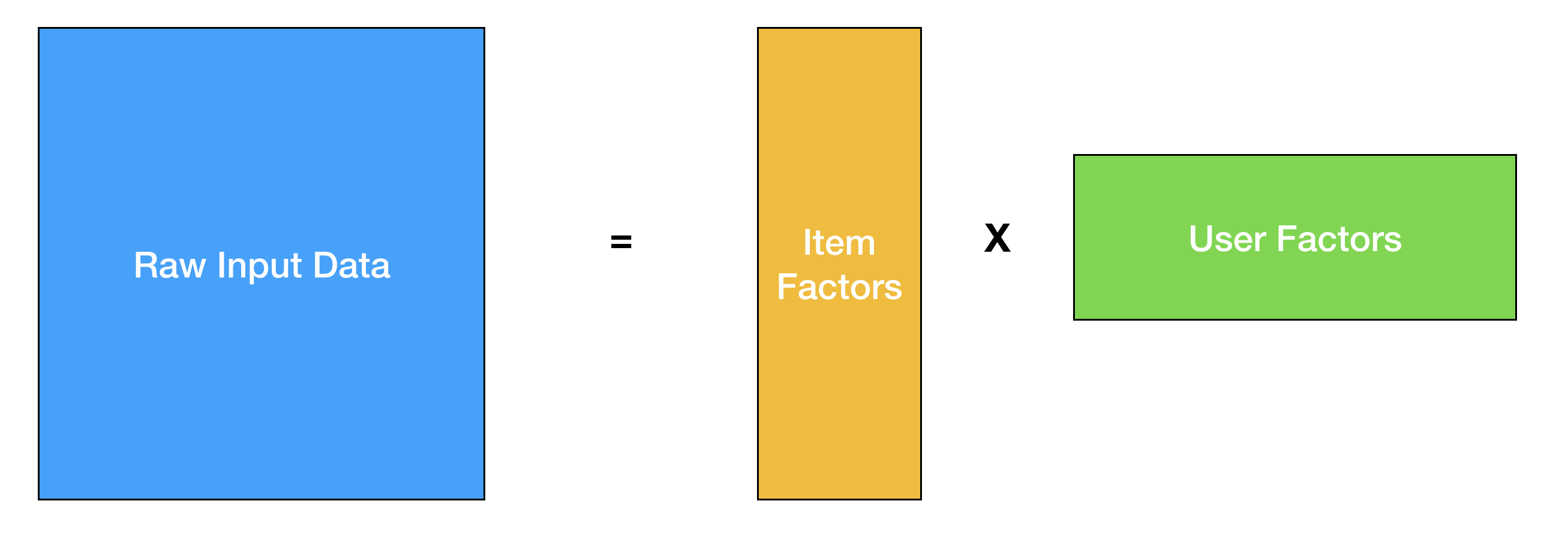
Once you have worked on different machine learning problems, most things in the field start to feel very similar. You take your raw input data, map it to a different latent space with fewer dimensions, and then perform your classification/regression/clustering. Recommender systems, new and old, are no different. In the classic collaborative filtering problem, you factorize your partially filled usage matrix to learn user-factors and item-factors, and try to predict user ratings with a dot-product of the factors.
This has worked well for many people at different companies and I have also had successes with it firsthand at Flipboard. And of course, people try to incorporate more signals into this model to get better performance for cold-start and other domain specific problems.
However, I didn’t really care about using fancy deep learning techniques for my recommendation problems until a friend asked me a very simple question at a conference a few years ago. If I recall correctly, he questioned my use of a certain regularizer, and I soon realized that his clever suggestion required me to go back to the whiteboard, recompute all the gradients and optimization steps, and essentially reimplement the core algorithm from scratch to test a relatively straightforward modification - I wasn’t writing PyTorch code, I only wished I did.
Enter AutoGrad and Embeddings
So, as it turns out the classic matrix-factorization problem can be formulated as a deep learning problem if you just think of the user-factors and item-factors as embeddings. An embedding is simply a mapping of a discrete valued list to a real valued lower dimensional vector (cough). Looking at the problem from this perspective gives you a lot more modelling flexibility thanks to the number of great autograd software out there. If you randomly initialize these embeddings, and define mean-squared-error as your loss, backpropagation would get you embeddings that would be very similar to what you would get with matrix factorization.
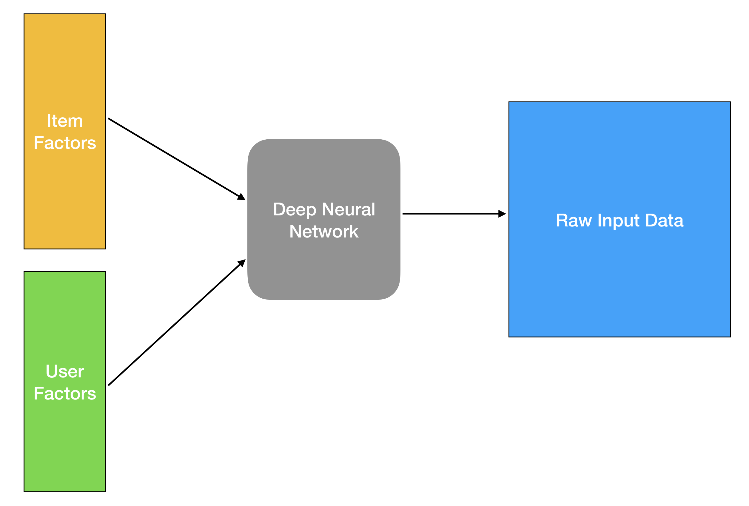
But as Justin Basilico showed in his informative ICML workshop talk, modelling the problem as a deep feed-forward network makes the learning task a lot trickier. Due to having more parameters and hyper-parameters, it requires more compute while only providing questionable improvements for the actual task. So why should we bother thinking of the problem in this way?
I would argue that modelling flexibility and experimentation ease are nothing to be scoffed at. This perspective allows you to incorporate all sorts of data into this framework fairly easily. Recommendation is also more than just predicting user-ratings, and you can solve many other recommendation problems such as sequence-aware recommendations a lot easier. Not to mention, because of autograd software, you end up with much shorter code that allows you to tweak things a lot quicker. I like optimizing my matrix-factorization with conjugate gradient as much as everyone else but please don’t ask me to recompute my CG steps after you add some new data and change your regularizer in the year 2020.
Other Ways To Learn Embeddings
The other great thing about embeddings is that there are several different ways of learning this mapping. If you don’t want to learn embeddings through random initialization and backpropagation from an input matrix, one very common approach is Skip-gram with negative-sampling. This method has been extremely popular in natural language processing, and has also been successful in creating embeddings from non-textual sequences such as graph-nodes, video games and Pinterest pins.
The core idea in skip-gram with negative sampling is to create a dataset with positive examples by sliding a context-window through a sequence and creating pairs of items that co-occur with a central item, and also generating negative data by random sampling items from the entire corpus, and create pairs of items that do not usually co-occur in the same window.
Once you have the dataset with both postive and negative examples, you simply train a classifier with a deep neural network and learn your embeddings. In this formulation, things that co-occur close to each other would have similar embeddings, which is usually what we need for most search and recommendation tasks.
For recommendation, there are many different ways to create these sequences. Airbnb has a great paper on how they collect sequences of listings based on a user’s sequential clicks of listings during a search/booking session to learn item-embeddings. Alibaba has another interesting way where they maintain an item-item interaction graph, where an edge from an item A to B indicates how often a user clicked on an item B after an item A, and then use random walks in the graph to generate sequences.
So What’s So Cool About These Embeddings?
In addition to the task at hand that each of those representations help solve (such as finding similar items), they are modular and amenable for transfer learning. One great thing about deep learning has been that you almost never have to start solving a problem from scratch, and all these different embeddings act as great places to start for new problems. If you wanted to build a new classifier (say, a spam detector), you could use your item embeddings as a starting point, and would be able to train a model much quicker with some basic fine-tuning.
These modular mappings to latent spaces have been extremely useful for me, and in addition to solving some recommendation problems, I have also been able to reuse and fine-tune these embeddings and solve many different end-tasks. Storing these embeddings in a centralized model storage further helps teams reduce redundancy and provides them with good foundations to build on for many problems.
While I hadn’t initially bought into the whole deep learning for recommender systems craze, I am starting to see beyond just the minimal performance gains on the original task, and highly recommend everyone to play around with this (still relatively new) paradigm in recommender systems!